6. Saving and managing sampling results
6.1. Accessing Sampled Data
The recommended way to access data from an MCMC run, irrespective of the
database backend, is to use the trace method:
>>> from pymc.examples import disaster_model
>>> from pymc import MCMC
>>> M = MCMC(disaster_model)
>>> M.sample(10)
Sampling: 100% [00000000000000000000000000000000000000000000000000] Iterations: 10
>>> M.trace('early_mean')[:]
array([ 2.28320992,  2.28320992,  2.28320992,  2.28320992,  2.28320992,
        2.36982455,  2.36982455,  3.1669422 ,  3.1669422 ,  3.14499489])
M.trace('early_mean') returns a copy of the Trace instance associated
with the tallyable object early_mean:
>>> M.trace('early_mean')
<pymc.database.ram.Trace object at 0x7fa4877a8b50>
Particular subsamples from the trace are obtained using the slice notation
[], similar to NumPy arrays. By default, trace returns the samples from
the last chain. To return the samples from all the chains, use chain=None:
>>> M.sample(5)
Sampling: 100% [000000000000000000000000000000000000000000000000000] Iterations: 5
>>> M.trace('early_mean', chain=None)[:]
array([ 2.28320992,  2.28320992,  2.28320992,  2.28320992,  2.28320992,
      2.36982455,  2.36982455,  3.1669422 ,  3.1669422 ,  3.14499489,
      3.14499489,  3.14499489,  3.14499489,  2.94672454,  3.10767686])
6.1.1. Output Summaries
PyMC samplers include a couple of methods that are useful for obtaining
summaries of the model, or particular member nodes, rather than the entire
trace. The summary method can be used to generate a pretty-printed summary
of posterior quantities. For example, if we want a statistical snapshot of the
early_mean node:
>>> M.early_mean.summary()

early_mean:

    Mean             SD               MC Error        95% HPD interval
    ------------------------------------------------------------------
    3.075            0.287            0.01             [ 2.594  3.722]


    Posterior quantiles:

    2.5             25              50              75             97.5
     |---------------|===============|===============|---------------|
    2.531            2.876           3.069          3.255         3.671
A method of the same name exists for the sampler, which yields summaries for every node in the model.
Alternatively, we may wish to write posterior statistics to a file, where they
may be imported into a spreadsheet or plotting package. In that case,
write_csv may be called to generate a comma-separated values (csv) file
containing all available statistics for each node:
M.write_csv("disasters.csv", variables=["early_mean", "late_mean", "switchpoint"])
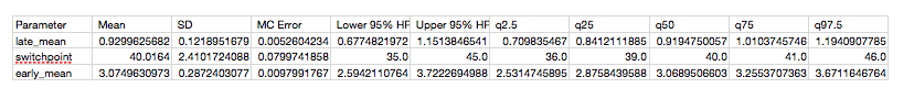
Summary statistics of stochastics from the disaster_model example,
shown in a spreadsheet.
write_csv is called with a single mandatory argument, the name of the
output file for the summary statistics, and several optional arguments,
including a list of parameters for which summaries are desired (if not
given, all model nodes are summarized) and an alpha level for calculating
credible intervalse (defaults to 0.05).
6.2. Saving Data to Disk
By default, the database backend selected by the MCMC sampler is the
ram backend, which simply holds the data in memory. Now, we will create a
sampler that instead will write data to a pickle file:
>>> M = MCMC(disaster_model, db='pickle', dbname='Disaster.pickle')
>>> M.db
<pymc.database.pickle.Database object at 0x7fa486623d90>
>>> M.sample(10)
>>> M.db.close()
Note that in this particular case, no data is written to disk before the call
to db.close. The close method will flush data to disk and prepare the
database for a potential session exit. Closing a Python session without
calling close beforehand is likely to corrupt the database, making the data
irretrievable. To simply flush data to disk without closing the database, use
the commit method.
Some backends not only have the ability to store the traces, but also the state of the step methods at the end of sampling. This is particularly useful when long warm-up periods are needed to tune the jump parameters. When the database is loaded in a new session, the step methods query the database to fetch the state they were in at the end of the last trace.
Check that you close() the database before closing the Python session.
6.3. Reloading a Database
To load a file created in a previous session, use the load function from
the backend:
>>> db = pymc.database.pickle.load('Disaster.pickle')
>>> len(db.trace('early_mean')[:])
10
The db object also has a trace method identical to that of Sampler.
You can hence inspect the results of a model, even when you don’t have the
model around.
To add a new trace to this file, we need to create an MCMC instance. This time,
instead of setting db='pickle', we will pass the existing Database
instance and sample as usual. A new trace will be appended to the first:
>>> M = MCMC(disaster_model, db=db)
>>> M.sample(5)
Sampling: 100% [000000000000000000000000000000000000000000000000000] Iterations: 5
>>> len(M.trace('early_model', chain=None)[:])
15
>>> M.db.close()
6.3.1. The ram backend
Used by default, this backend simply holds a copy in memory, with no output written to disk. This is useful for short runs or testing. For long runs generating large amount of data, using this backend may fill the available memory, forcing the OS to store data in the cache, slowing down all other applications.
6.3.2. The no_trace backend
This backend simply does not store the trace. This may be useful for testing purposes.
6.3.3. The txt backend
With the txt backend, the data is written to disk in ASCII files. More
precisely, the dbname argument is used to create a top directory into which
chain directories, called Chain_<#>, are going to be created each time
sample is called:
dbname/
  Chain_0/
    <object0 name>.txt
    <object1 name>.txt
    ...
  Chain_1/
    <object0 name>.txt
    <object1 name>.txt
    ...
  ...
In each one of these chain directories, files named <variable name>.txt are
created, storing the values of the variable as rows of text:
# Variable: e
# Sample shape: (5,)
# Date: 2008-11-18 17:19:13.554188
3.033672373807017486e+00
3.033672373807017486e+00
...
While the txt backend makes it easy to load data using other applications and programming languages, it is not optimized for speed nor memory efficiency. If you plan on generating and handling large datasets, read on for better options.
6.3.4. The pickle backend
The pickle database relies on the cPickle module to save the traces.
Use of this backend is appropriate for small-scale, short-lived projects. For
longer term or larger projects, the pickle backend should be avoided since
generated files might be unreadable across different Python versions. The
pickled file is a simple dump of a dictionary containing the NumPy arrays
storing the traces, as well as the state of the Sampler‘s step methods.
6.3.5. The sqlite backend
The sqlite backend is based on the python module sqlite3 (built-in to
Python versions greater than 2.4) . It opens an SQL database named dbname,
and creates one table per tallyable objects. The rows of this table store a
key, the chain index and the values of the objects:
key (INTT), trace (INT), v1 (FLOAT), v2 (FLOAT), v3 (FLOAT) ...
The key is autoincremented each time a new row is added to the table, that is,
each time tally is called by the sampler. Note that the savestate
feature is not implemented, that is, the state of the step methods is not
stored internally in the database.
6.3.6. The hdf5 backend
The hdf5 backend uses pyTables to save data in binary HDF5 format. The
hdf5 database is fast and can store huge traces, far larger than the
available RAM. Data can be compressed and decompressed on the fly to reduce the
disk footprint. Another feature of this backends is that it can store arbitrary
objects. Whereas the other backends are limited to numerical values, hdf5
can tally any object that can be pickled, opening the door for powerful and
exotic applications (see pymc.gp).
The internal structure of an HDF5 file storing both numerical values and arbitrary objects is as follows:
/ (root)
  /chain0/ (Group) 'Chain #0'
    /chain0/PyMCSamples (Table(N,)) 'PyMC Samples'
    /chain0/group0 (Group) 'Group storing objects.'
      /chain0/group0/<object0 name> (VLArray(N,)) '<object0 name> samples.'
      /chain0/group0/<object1 name> (VLArray(N,)) '<object1 name> samples.'
      ...
  /chain1/ (Group) 'Chain #1'
    ...
All standard numerical values are stored in a Table, while objects are
stored in individual VLArrays.
The hdf5 Database takes the following parameters:
dbname(string) Name of the hdf5 file.dbmode(string) File mode:a: append,w: overwrite,r: read-only.dbcomplevel(int (0-9)) Compression level, 0: no compression.dbcomplib(string) Compression library (zlib,bzip2,lzo)
According the the pyTables manual, zlib ([Roelofs2010]) has a fast decompression, relatively slow compression, and a good compression ratio. LZO ([Oberhumer2008]) has a fast compression, but a low compression ratio. bzip2 ([Seward2007]) has an excellent compression ratio but requires more CPU. Note that some of these compression algorithms require additional software to work (see the pyTables manual).
6.4. Writing a New Backend
It is relatively easy to write a new backend for PyMC. The first step is to
look at the database.base module, which defines barebone Database and
Trace classes. This module contains documentation on the methods that
should be defined to get a working backend.
Testing your new backend should be trivial, since the test_database module
contains a generic test class that can easily be subclassed to check that the
basic features required of all backends are implemented and working properly.